Understanding Of Different Filter Design and its Properties

 

Understanding Filter Design and its Properties

Objective:

Aim of this topic is to analyze a given system (FIR and IIR Filters) and find its various properties such as magnitude response, phase response and group delay etc. on the bases of z-transform.

Description:

There are different parameters on the bases of which we can analyze a system or signal in DSP, some of them are listed below:

·         Magnitude Response

·         Phase Response

·         Impulse Response

·         Group Delay

·         Pole Zero Plot

Magnitude Response:

The amplitude response   of an LTI filter is defined as the magnitude (or modulus) of the (complex) filter frequency response   , i.e.,

Another common name for the amplitude response is magnitude frequency response.

The real-valued amplitude response   specifies the amplitude gain that the filter provides at each frequency   .

No digital filter is ideal and therefore they will always a have smooth (rather than a clearly defined or discontinuous) transition between the pass and stop bands at the cutoff frequency  .

The cutoff frequency is typically defined as the frequency at which the power transmitted by the filter drops to one-half (by -3 dB) of the maximum power transmitted in the passband.

 

Phase Response:

In signal processing and electrical engineering, phase response is the relationship between the phase of a sinusoidal input and the output signal passing through any device that accepts input and produces an output signal, such as an amplifier or a filter.

Amplifiers, filters, and other devices are often categorized by their amplitude and/or phase response. The amplitude response is the ratio of output amplitude to input, usually a function of the frequency. Similarly, phase response is the phase of the output with the input as reference. The input is defined as zero phase. A phase response is not limited to lying between 0° and 360°, as phase can accumulate to any amount of time.

Group Delay:

In signal processing, group delay is a measure of the time delay of the amplitude envelopes of the various sinusoidal components of a signal through a device under test, and is a function of frequency for each component. Phase delay is a similar measure of the time delay of the phase, instead of the delay of the amplitude envelope, of each sinusoidal component.

All frequency components of a signal are delayed when passed through a device such as an amplifier, a loudspeaker, or propagating through space or a medium, such as air. This signal delaywill be different for the various frequencies unless the device has the property of being linear phase. (Linear phase and minimum phase are often confused. They are quite different.) The delay variation means that signals consisting of multiple frequency components will suffer distortion because these components are not delayed by the same amount of time at the output of the device. This changes the shape of the signal in addition to any constant delay or scale change. A sufficiently large delay variation can cause problems such as poor fidelity in audio or inter-symbol interference(ISI) in the demodulation of digital information from an analog carrier signal. High speed modems use adaptive equalizers to compensate for non-constant group delay.

Pole-Zero Plots:

In mathematics, signal processing and control theory, a pole–zero plot is a graphical representation of a rational transfer function in the complex plane which helps to convey certain properties of the system such as:

o   Stability

o   Causal system / anti-causal system

o   Region of convergence (ROC)

o   Minimum phase / non minimum phase

A pole-zero plot shows the location in the complex plane of the poles and zeros of the transfer function of a dynamic system, such as a controller, compensator, sensor, equalizer, filter, or communications channel. By convention, the poles of the system are indicated in the plot by an X while the zeroes are indicated by a circle or O.

A pole-zero plot can represent either a continuous-time (CT) or a discrete-time (DT) system. For a CT system, the plane in which the poles and zeros appear is the s plane of the Laplace transform. In this context, the parameter s represents the complex angular frequency, which is the domain of the CT transfer function. For a DT system, the plane is the z plane, where z represents the domain of the Z-transform.

Filter Types:

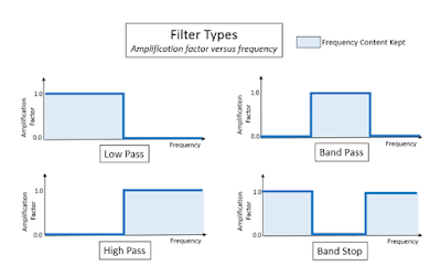
High Pass – High pass filter is used to remove low frequency offsets from a signal. For example, if interested in only the dynamic content of a strain gauge signal, any low frequency drift in a gauge could be removed with a high pass filter.

Low Pass - A low pass filter attenuates, or gets rid of, frequencies above a specified frequency. For example, this could be used to remove high frequency hiss from an audio recording.

Band Pass – This filter is used to allow only a band limited portion of the frequency content to be passed through the filter.

Band Stop – A band stop filter is used to remove frequency content over a specified range.

These filter types can be implemented using either FIR or IIR filters. It is also possible to use a combination of these to produce an arbitrary shaped filter.

Infinite Impulse Response (IIR) Filters:-

Another type of filter is the Infinite Impulse Response (IIR) filter and the Impulse Response of an IIR filter is of infinite duration. The IIR filters have the feedback, due to which they are also known as Recursive filters. The general difference for an IIR filter is:

Where,

Where "ak" is the k-th feedback tap. The left "Σ" denoted the summation from k =1 to k =N-1, "N" is the number of the feedback taps in the IIR filter. The right "Σ" denotes the summation from k = 0 to k = M – 1, where "M" is the number of feedforward taps. We have given the codes for IIR filter design using Butterworth, Chebyshev Type I, Chebyshev Type II and Elliptic Filters.

Finite Impulse Response (FIR) Filters:-

A Finite Impulse Response (FIR) filter is the one filters whose impulse response is of finite duration. The FIR filters do not have the feedback, due to which they are also known as Non-Recursive filters. The general difference equation for a FIR filter is:

Where "y(n)" is the filter output at discrete time instances "n", "bk" is the k-th feedforward tap, or the filter coefficient, and "x(n – k)" is the filter input delayed by "k" samples. The "Σ" denotes summation from k = 0 to k = M -1, where "M" is the number of the feedforward taps in the FIR filter. Note that the FIR filter output depends only on the previous "M" inputs. This feature is why the impulse response for a FIR filter is finite.

FIR filters have some drawbacks, however. The most important is that they can be computationally expensive to implement. Another is that they have a long transient response. It is commonly thought that IIR filters must be used when computational power is at the premium. This is certainly true is some case. However, in many cases, the use of multistage or multirate techniques can yield FIR implementations that can compete (and even surpass) IIR implementations while retaining the nice characteristics of FIR filters such as linear phase, stability, and robustness to quantization effects. However, these efficient multistage or multirate designs tend to have very large transient responses, so depending on the requirements of the filter, IIR design may still be the way to go.

Here is the practical problem to solve let start:

01. Perform the following.

a)      Find the coefficients of 10^th order difference equation for a low pass filter using filter design toolbox.  

b)     Plot frequency response, magnitude, phase and group delay of the filter.

c)      Plot a pole-zero plot of the filter.

d)     Plot first 200 samples of impulse response of the filter.

e)      Read a voice file and plot the magnitude of the signal before and after passing it through filter.

 

Be creative and demonstrate the effect by group delay of the filter by generating a signal with multiple frequencies and pass it through the filter. 

CODE:

function Hd = firii

Fs = 8000;    % Sampling Frequency

N     = 10;   % Order

Fpass = 300;  % Passband Frequency

Fstop = 800;  % Stopband Frequency

Wpass = 1;    % Passband Weight

Wstop = 80;   % Stopband Weight

dens  = 20;   % Density Factor

 

% Calculate the coefficients using the FIRPM function.

b  = firpm(N, [0 Fpass Fstop Fs/2]/(Fs/2), [1 1 0 0], [Wpass Wstop], ...

           {dens});

Hd = dfilt.dffir(b);

 

%first 200 samples of impulse response

impz(Hd,200)

%frequency response of the filter

freqz(Hd)

rec = audiorecorder(8000,8,1);      %audio recorded at 8k Hz

record(rec,3);                      %record for 3 seconds

input =getaudiodata(rec);           %generate audio data   

Fs =8000;                           %sampling frequency

T = 1/Fs;                           %Time period   

Output = filter(Hd,input) ;         %pass through filter

% sound(Output,Fsam)

figure

%plot input and filtered signals in time domain

subplot(2,1,1)

t = 0:T:(length(input)*T)-T;

plot(t,input)

title('Original Signal in Time Domain')

xlabel('Time')

ylabel('Amplitude')

subplot(2,1,2)

t = 0:T:(length(Output)*T)-T;

plot(t,Output)

title('Filtered Signal in Time Domain')

xlabel('Frequency')

ylabel('Amplitude')

 

figure

%plot input and filtered signals in frequency domain

subplot(2,1,1)

FFTin= abs(fft(input));

f = (0:length(FFTin)-1)*Fs/length(FFTin);

plot(f,FFTin)

title('Original Signal in Frequency Domain')

xlabel('Frequency')

ylabel('Magnitude')

subplot(2,1,2)

Out_fft = abs(fft(Output));

fo = (0:length(Out_fft)-1)*Fs/length(Out_fft);

plot(fo,Out_fft)

title('Filtered Signal in Frequency Domain')

xlabel('Frequency')

ylabel('Magnitude')

FILTER DESIGN:

 

 

FILTER COEFFICIENTS:

 

 

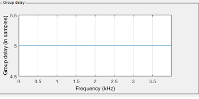
GROUP DELAY:

In this case, group delay is a constant value of 5 samples. Since the filter is FIR, the group delay will be constant for all the frequency values.

 

 

 

IMPULSE RESPONSE (200 SAMPLES):

Since the filter is an FIR, it exhibits symmetrical impulse response. It can be seen that it is shifted by 5 due to the group delay of 5

 

 

FREQUENCY RESPONSE:

 

 

 

 

 

 

 

 

 

 

 

MAGNITUDE RESPONSE:

 

 

PHASE RESPONSE:

 

 

 

PHASE DELAY:

 

 

POLE ZERO PLOT:

 

 

OUTPUT:

After passing through the low pass filter, the audio sounded very diminished due to loss of high frequency contents.

 

As clear from the frequency domain analysis, the high frequency contents are attenuated after being passed from the low pass filter.

 

Passing a sinusoid of 4 varying frequencies passed through the loss pass filter generated in Task 1 Part b

CODE:

function Hd = firtwo

% All frequency values are in Hz.

Fs = 8000;  % Sampling Frequency

N     = 10;    % Order

Fpass = 1000;  % Passband Frequency

Fstop = 2000;  % Stopband Frequency

Wpass = 1;     % Passband Weight

Wstop = 80;    % Stopband Weight

dens  = 20;    % Density Factor

% Calculate the coefficients using the FIRPM function.

b  = firpm(N, [0 Fpass Fstop Fs/2]/(Fs/2), [1 1 0 0], [Wpass Wstop], ...

           {dens});

Hd = dfilt.dffir(b);

Fs=800

%define three frequencies

f1 = 600;

f2 = 1200;

f3 = 1800;

f4 = 2400;

T =1;   %Time period

dt =1/Fs;

t = 0:dt:T;

%Three sines with different frequencies

Signal_1 = sin(2*pi*f1*t);     

Signal_2 = sin(2*pi*f2*t);

Signal_3 = sin(2*pi*f3*t);

Signal_4 = sin(2*pi*f4*t);

figure

%add the signals

Group = Signal_1+Signal_2+Signal_3+Signal_4;

%pass the signals through the filter simultaneously

Filtered_Output = filter(Hd,Group);

figure

%plot the signal before and after passing through the filter in time domain

subplot(2,1,1)

plot(Group)

xlim([0 800])

title('Before Applying Filter')

xlabel('Time')

ylabel('Amplitude')

subplot(2,1,2)

plot(Filtered_Output)

xlim([0 800])

title('After Applying Filter')

xlabel('Time')

ylabel('Amplitude')

figure

%plot the signal before and after passing through the filter in frequency domain

subplot(2,1,1)

Group_F  = abs(fft(Group));

fg = (0:length(Group_F)-1)*Fs/length(Group_F);

plot(fg,Group_F)

title('Original Signal in Frequency Domain')

xlabel('Frequency')

ylabel('Magnitude')

subplot(2,1,2)

FilteredOutput_F  = abs(fft(Filtered_Output));

fg = (0:length(FilteredOutput_F)-1)*Fs/length(FilteredOutput_F);

plot(fg,FilteredOutput_F)

title('Filtered Signal in Frequency Domain')

xlabel('Frequency')

ylabel('Magnitude')

 

OUTPUT: